Training Material for Your
MBA Finance™ Degree

MBA Finance™ Training

Nature and Importance of the Finance Function
Functions of the Finance Manager
Interface Between Finance and Other Business Functions
Environment of Corporate Finance
Time Value for Money
The Measure of Return
Sources of Financial Risks
Financial Portfolios and Risks
Financial Risk Management
Risk Management Process

Register Your MBA Degree >>

Nature and Importance of the Finance Function

In this chapter, you will:

Understand the nature and importance of the finance function
Understand the various objectives of financial management

One participant in a course titled, ‘Finance for Non-Finance Executives’, made a very interesting observation during the discussion. He said, “There are no executive development programs titled ‘Production Management for Non-Production Executives’ or ‘Marketing Management for Non-Marketing Executives’ and so on. Then how come books and Executive Development Programs titled ‘Finance for Non-Finance Executives’ are so popular among managers of all functions like marketing, production, personnel, R&D, etc.?”

The answer is very simple. The common thread running through all the decisions taken by the various managers is money and there is hardly any manager working in any organization to whom money does not matter. To illustrate this point, let us consider the following instances.

The R&D manager has to justify the money spent on research by coming up with new products and processes which would help to reduce costs and increase revenue. If the R&D department is like a bottomless pit only swallowing more and more money but not giving any positive results in return, then the management would have no choice but to close it. No commercial entity runs a R&D department to conduct infructuous basic research.
Likewise the materials manager should be aware that inventory of different items in stores is nothing but money in the shape of inventory. He should make efforts to reduce inventory so that the funds released could be put to more productive use. At the same time, he should also ensure that inventory of materials does not reach such a low level as to interrupt the production process. He has to achieve the right balance between too much and too little inventory. This is called the liquidity- proﬁtability trade-off about which you will read more in the lessons on Working Capital Management. The same is true with regard to every activity in an organization. The results of all activities in an organization are reﬂected in the ﬁnancial statements in dollars. The Finance Manager (you), as your very designation implies, should be involved in all financial matters of the organization since almost all activities in the organization have ﬁnancial implications. It would therefore not be inaccurate to say that the Finance Manager is involved in most decisions of the organization. Let us try to understand what ﬁnancial management is by examining what the Finance Manager does and with what objectives.
Objective of Financial Management
Let us examine the purpose or objective sought to be achieved by a Finance Manager. Suppose you manage to make available the required funds at an acceptable cost and that the funds are suitably invested and that everything goes according to plan because of the effective control measures employed by you. If the ﬁrm is a commercial or proﬁt-seeking ﬁrm, then the results of good performance are reflected in the proﬁts the ﬁrm earns. How are the proﬁts utilized? They are partly distributed among the owners as dividends and partly recycled into the operations of the ﬁrm. As this process continues over a period of time the value of the ﬁrm increases for the simple reason that the ﬁrm is able to generate attractive surpluses from operations. If the shares of a ﬁrm are traded on the stock exchange, the good performance of the ﬁrm is reﬂected in the price at which its shares are traded. When the ﬁrm’s shares attract a good price, the owners or shareholders are better off because they would realize much more than what they had invested. Their wealth increases. So we can see that as a result of good ﬁnancial management the value of the company to the owners (shareholders) increases, thereby increasing their wealth. Therefore, we can say that your objective as a Finance Manager is to increase or maximize the wealth of the owners by increasing the value of the ﬁrm which is reflected in its Earnings per Share (EPS) and the market price of its shares.

In the case of public sector companies, till recently the only objective was to increase the wealth to the society and nation at large. This objective was achieved by ensuring availability of essential goods and services to all citizens in all corners of the country, uniform development of all regions in the country, providing employment opportunities, investing in projects with long gestation periods where private investment may not be forthcoming and investing in import-substitution industries, etc. But now the public sector has also come to realize that they have to perform in order to exist and that its products/services will not be subsidized any longer by the government. Public Sector Undertakings (PSUs) are now going in for disinvestment and privatization for increased efficiency.

Summary:

The Finance Manager should be involved in all financial matters of the organization since almost all activities in the organization have ﬁnancial implications.
If the ﬁrm is a commercial or proﬁt-seeking ﬁrm, then the results of good performance are reflected in the proﬁts the ﬁrm earns.
As this process continues over a period of time the value of the ﬁrm increases for the simple reason that the ﬁrm is able to generate attractive surpluses from operations.
Public Sector Undertakings (PSUs) are now going in for disinvestment and privatization for increased efficiency.

Functions of the Finance Manager

In this chapter, you will:

Understand the process of deployment of funds
Understand finance manager’s control over the use of organization’s funds
Also understand the risk vs return trade-off

As finance manager, you have to plan for and mobilize the required funds from various sources when they are required and at an acceptable cost. This decision is called the Financing Decision. For this purpose you would be liaising with banks and financial institutions. You also deal with merchant banking agencies for procuring funds from the public through issue of shares, debentures and inviting the public to subscribe to its fixed deposits. In deciding how much to procure from various sources, you would weigh many considerations like the cost of the funds in the form of interest / dividend and the cost of public issue in the case of shares and debentures, the length of time for which funds would be available, etc. Banks and other ﬁnancial institutions which give short-term and long-term loans generally lay down some conditions. These conditions are aimed at ensuring the safety of the loans given by them and contain provisions restricting the freedom of the borrower to raise loans from other sources. Therefore, as Finance Manager, you would try to balance the advantages of having funds available with the costs and the loss of ﬂexibility arising from the restrictive provisions of the loan contract.

Let us take a look at a real life example:

XYZ Limited, a well-known company in computer training, software development. Information systems, consultancy, etc. is undertaking a modernization cum expansion scheme which envisages addition of new services, product lines and upgradation of existing systems. The cost of this expansion cum modernization program is estimated at $357.8 million, which is going to be mobilized as follows as per the prospectus of the company.

*Item*	*Cost ($ MM)*
Public issue of equity shares including premium Term Loan Leasing Others Deferred payment guarantee Internal accruals	180.4 13 12.5 7.5 9.9 134.5
TOTAL:	357.8

Functions of the Finance Manager

Deployment of Funds
There are always many competing needs for the allocation of funds. In consultation with the managers of various departments such as production, marketing, personnel, R&D and the top management you (the Finance Manager) decide on the manner of deployment of funds in various assets such as land, buildings, machinery, materials, etc. Sometimes the managers of the various departments named above constitute an ‘Investment Committee’ and appraise an investment proposal along the marketing, technical and ﬁnancial dimensions. You appraise the proposal along the ﬁnancial dimensions to determine its worthiness in relation to the investment involved. This decision called the ‘Investment Decision’ constitutes one of the core activities of your role as a Finance Manager.

The funds mobilized through various sources by XYZ are proposed to be deployed as follows, as indicated in the prospectus of the company.

*Item*	*Cost ($ MM)*
Building Computers & Accessories Plant & Machinery Infrastructure Normal Capital Expenditure Repayment of Loans Increase in Working Capital	98.5 94.1 11.6 21.3 24.1 28.3 79.9
TOTAL:	357.8

Control Over the Use of Funds
After deciding on projects and proposals in which the funds are to be invested and after procuring them, you have to continuously monitor their use in order to ensure that procurement and deployment of funds proceeds according to plan. This task of the Finance Manager is called Financial Control. You send frequent reports to the Managing Director. These reports contain information in the form of facts and figures regarding the extent to which procurement and deployment of funds is proceeding according to plan. For example, the reports would inform the management regarding the extent to which credit sanctioned by banks for the day-to-day use of the ﬁrm (working capital) has been utilized and how much more can be borrowed. It would also contain information on how much money is due to the firm from various customers and how much the ﬁrm owes its suppliers. The report would also contain information on the funds required at different points of time in the future and the availability of funds from various sources including those available out of any surpluses generated internally. You would also be reporting to the top management about the performance of individual departments within the organization. All such reports are called ‘Control Reports’ and the whole process constitutes ‘control’ because it helps management to take timely corrective action to ensure that planned results are achieved.

Risk-return Trade-off
While making the decisions regarding investment and ﬁnancing, as Finance Manager, you seek to achieve the right balance between risk and return. If the firm borrows heavily to ﬁnance its operations, then the surpluses generated out of operations would be utilized to ‘Service the Debt’ in the form of interest and principal payments. The surplus or profit available to the owners would be reduced because of the heavy ‘Debt-servicing’. If things do not work out as planned and the ﬁrm is unable to meet its obligations, the company is even exposed to the risk insolvency. Similarly, the various investment opportunities have a certain amount of risk associated with the return and also the time when the return would materialize. You have to decide whether the opportunity is worth more than its cost and whether the additional burden of debt can be safely borne. In fact, decision making in all areas of management including ﬁnancial management involves the balancing of the trade-off between risk and return.

Summary:

The Finance Manager has to plan for and mobilize the required funds from various sources when they are required and at an acceptable cost. This decision is called the Financing Decision.
The Finance Manager would try to balance the advantages of having funds available with the costs and the loss of ﬂexibility arising from the restrictive provisions of the loan contract.
The Finance Manager appraises the proposal along the ﬁnancial dimensions to determine its worthiness in relation to the investment involved. This decision called the ‘Investment Decision’ constitutes one of the core activities of the Finance Manager.
After deciding on projects and proposals in which the funds are to be invested and after procuring them, the Finance Manager has to continuously monitor their use in order to ensure that procurement and deployment of funds proceeds according to plan. This task of the Finance Manager is called Financial Control.
While making the decisions regarding investment and ﬁnancing, the Finance Manager seeks to achieve the right balance between risk and return.

Interface Between Finance and Other Business Functions

In this chapter, you will:

Understand the interface between finance and:
- The Marketing Function
- The Production Function
- The Top Management
Understand other challenges in Financial Management including:
- Treasury Operations
- Foreign Exchange
- Financial Structuring
- Maintaining Share prices
- Ensuring Management Control

Let us discuss in greater detail the reasons why knowledge of the ﬁnancial implications of the ﬁnance manager’s decisions is important to the non-ﬁnance managers. One common factor among all managers is that they use resources and since resources are obtained in exchange for money, they are in effect making the investment decision and in the process of ensuring that the investment is effectively utilized they are also performing the control function.

Interfaces of Finance with other Business Functions

Marketing – Finance Interface
The Marketing Manager takes many decisions which have a signiﬁcant impact on the proﬁtability of the ﬁrm. For example, he should have a clear understanding of the impact of the credit extended to the customers on the proﬁts of the company. Otherwise in his eagerness to meet the sales targets he is likely to extend liberal terms of credit which may put the proﬁt plans out of gear. Similarly, he should weigh the beneﬁts of keeping a large inventory of ﬁnished goods in anticipation of sales against the costs of maintaining that inventory. Other key decisions of the Marketing Manager which have ﬁnancial implications are pricing, product, promotion and advertisement, choice of product mix and distribution policy.

Production – Finance Interface
In any manufacturing ﬁrm, the Production Manager controls a major part of the investment in the form of equipment, materials and men. He should so organize his department that the equipments, under his control are used most productively, the inventory of work-in-process or unﬁnished goods and stores and spares is optimized and the idle time and work stoppages are minimized. If the production manager can achieve this, he would be holding the cost of the output under control and thereby help in maximizing proﬁts. He has to appreciate the fact that whereas the price at which the output can be sold is largely determined by factors external to the firm like competition, government regulations, etc. the cost of production is more amenable to his control. Similarly, he would have to make decisions regarding make or buy, buy or lease, etc. for which he has to evaluate the ﬁnancial implications before arriving at a decision.

Top Management – Finance Interface
The top management, which is interested in ensuring that the ﬁrm’s long-term goals are met, ﬁnds it convenient to use the ﬁnancial statements as a means for keeping itself informed of the overall effectiveness of the organization. We have so far brieﬂy reviewed the interface of ﬁnance with the non-ﬁnance functional disciplines like production, marketing, etc. Besides these, the ﬁnance function also has a strong linkage with the functions of the top management. Strategic planning and management control are two important functions of the top management. Finance function provides the basic inputs needed to undertake these activities.

With the recent liberalization of many economies, abolition of the ofﬁce of the Controller of Capital Issues who used to ﬁx issue prices beforehand and efforts of these economies towards globalization, ﬁnance managers are presently facing some new challenges as indicated below:

Other Challenges in Financial Management
Treasury Operations:
Short-term fund management must be more sophisticated. As finance manager, you could make speculative gains by anticipating interest rate movements.

Foreign Exchange:
You will have to weigh the costs and beneﬁts of transacting in foreign exchange particularly now that most of the economies are going global and the future value of the currencies is becoming difﬁcult to predict.

Financial Structuring:
An optimum mix between debt and equity will be essential. Firms will have to tailor ﬁnancial instruments to suit their and investors’ needs. Pricing of new issues is an important task for the Finance Manager’s portfolio now.

Maintaining Share Prices:
In the premium equity era, ﬁrms must ensure that share prices stay healthy. You will have to devise appropriate dividend and bonus policies.

Ensuring Management Control:
Equity issues at premium mean management may lose control if it is unable to take up its share entitlements. Strategies to prevent this are vital.

Summary:

Marketing-finance interface:
- A finance manager should weigh the beneﬁts of keeping a large inventory of ﬁnished goods in anticipation of sales against the costs of maintaining that inventory.
- Other key decisions are pricing, product, promotion and advertisement, choice of product mix and distribution policy.
Production-finance interface:
- The production manager should so organize his department that the equipment’s, under his control are used most productively, the inventory of work-in-process or unﬁnished goods and stores and spares is optimized and the idle time and work stoppages are minimized.
Top management-finance interface:
- Strategic planning and management control are two important functions of the top management. Finance function provides the basic inputs needed to undertake these activities.
Other Challenges in Financial Management:
- Treasury Operations
- Foreign Exchange
- Maintaining Share Prices
- Ensuring Management Control

Environment of Corporate Finance

In this chapter, you will:

Understand the environment of corporate finance
Understand the important forms of business organization
- Sole Proprietorship
- Partnership
- Companies

One of the important aspects of your job as a Finance Manager is to understand the external environment in which you operate. In a country where investment and ﬁnancing activities are subject to numerous governmental controls and legislations, you must have a thorough understanding of the legal framework circumscribing his decisions. Let us consider the following examples to clarify the point:

Colgate is the market leader in dental products (toothpaste and tooth powder) and it can increase its market share by increasing production. But the ﬁnance manager of Colgate cannot recommend a proposal for expanding the manufacturing capacity of toothpaste even though the project is certain to increase the shareholders’ wealth. Why? Because in most countries toothpaste manufacture is an activity reserved for the small scale sector and the government does not permit units other than small-scale units engaged in this activity to expand their capacity.
The confectionery products of Nutrine enjoy a strong brand image. Its ﬁnance manager would possibly like to exploit this strength for raising funds from public through issue of shares. But he cannot resort to this option even if he so desires because Nutrine is a private limited company and the Companies Act in many countries prohibits private limited companies from raising capital from the public.

From these examples, it is clear that the legislative framework has an important bearing on the investment and ﬁnancing decisions of a ﬁrm. The next question is: Are there external factors other than legal provisions and governmental regulations that that intervene in the decision making process of the ﬁnance manager? The answer is ‘Yes’. The form of organization that business entity adopts often limits the investment and ﬁnancing options. For instance, a partnership ﬁrm engaged in trading yarn cannot follow Castrol and set up a $4000 MM petrochemical complex because the partnership form of organization limits both the size and the ability to mobilize such massive funds.

The structure of the ﬁnancial markets from where you have to raise funds and the regulations governing the ﬁnancial intermediaries (like banks and ﬁnancial institutions) also influence your decisions as ﬁnance manager. Last but not the least in terms of importance is the tax factor. While evaluating the feasibility of the investments you also take into account the ﬁscal (tax) factors associated with these investments.

So, we ﬁnd that you pursue your objective of owners’ wealth maximization under a set of external constraints apart from the internal constraints that arise from the inherent strengths and weaknesses of each entity. This makes your job complex and interesting because he has to make optimal decisions within the framework of these constraints.

We have identiﬁed four aspects of the external environment which are directly relevant to your job as Finance Manager. They are:

Forms of Business Organization.
Regulatory Framework.
Financial System (which will include ﬁnancial markets and intermediaries).
Tax Aspects.

The Important Forms of Business Organization

Important Forms of Business Organizations

Solo Proprietorship
This type of concern is owned by a single person. The proprietor enjoys all the powers of taking and assuming risks for his/her concern. The rewards, proﬁts, losses and incurring of all the liabilities of the business is to him/her.

The advantages of a sole proprietorship are:

Easy and inexpensive to set up.
Few governmental regulations.
No ﬁrm tax.

The disadvantages are:

Life of the ﬁrm is limited to the life of the owner.
Unlimited personal liabilities.
Outside fund raising is not possible and can result in lack of growth.
Tax on the income will be very high.

Partnership
In this type of ﬁrm the business is owned by two or more persons. They are partners in business and they bear the risks and reap the rewards of the business.

The partnership comes into being through a partnership agreement or a partnership deed.

The advantages of the partnership ﬁrm are:

Like a sole ownership ﬁrm it can be set up easily and inexpensively.
It is relatively free from governmental regulations.
The expertise and experience of the partners is useful to the ﬁrm’s operations.

The disadvantages are:

The life of the ﬁrm depends upon the agreement between the partners. If any of them withdraws or is met with death, it may result in dissolution of the ﬁrm.
Possible conﬂict between the partners is a threat to the company’s existence.
Personal liabilities of the partners is unlimited.
Its ability to raise funds is limited.

Companies
A group of persons working together towards a common objective is a company. It represents different kinds of associations, be it business or non-business. Details about company structures are specified by the Chamber of Commerces of respective countries.

Summary:

A ﬁnance manager must have a thorough understanding of the legal framework circumscribing his decisions.
The structure of the ﬁnancial markets from where the ﬁnance manager has to raise funds and the regulations governing the ﬁnancial intermediaries (like banks and ﬁnancial institutions) also influence the decisions of a ﬁnance manager.
Important Forms of Business Organization include:
- Sole Proprietorship: This type of concern is owned by a single person.
- Partnership: In this type of ﬁrm the business is owned by two or more persons.
- Companies: A group of persons working together towards a common objective is a company.

Time Value for Money

In this chapter, you will:

Understand the process of compounding
Understand the process of discounting
Understand the future value of single flow (lump sum)
Understand what is doubling period
Understand what is growth rate

To keep pace with the increasing competition, companies have to go in for new ideas implemented through new projects be it for expansion, diversiﬁcation or modernization. A project is an activity that involves investing a sum of money now in anticipation of beneﬁts spread over a period of time in the future. How do you determine whether the project is ﬁnancially viable or not? Your immediate response to this question will be to sum up the beneﬁts accruing over the future period and compare the total value of the beneﬁts with the initial investment. If the aggregate value of the beneﬁts exceeds the initial investment, the project is considered to be ﬁnancially viable.

While this approach prima facie appears to be satisfactory, you must be aware of an important assumption that underlies. You have assumed that irrespective of the time when money is invested or received, the value of money remains the same. Put differently, you have assumed that: value of one dollar now = value of one dollar at the end of year 1 = value of one dollar at the end of year 2 and so on. You know intuitively that this assumption is incorrect because money has time value. How do you deﬁne this time value of money and build it into the cash flows of a project? The answer to this question forms the subject matter of this chapter.

You intuitively know that $1000 in hand now is more valuable than $1000 receivable after a year. In other words, you will not part with $1000 now in return for a ﬁrm assurance that the same sum will be repaid after a year. But you might part with $1000 now if you are assured that something more than $1000 will be paid at the end of the ﬁrst year. This additional compensation required for parting with $1000 now is called ‘interest’ or the time value of money. Normally, interest is expressed in terms of percentage per annum for example, 12 percent p.a. or 18 percent p.a. and so on.

Why should money have time value? Here are some important reasons for this phenomenon:

Money can be employed productively to generate real returns. For instance, if a sum of $100 invested in raw material and labor results in ﬁnished goods worth $105, you can say that the investment of $100 has earned a rate of return of 5 percent.

In an inflationary period, a dollar today has a higher purchasing power than a dollar in the future.

Since future is characterized by uncertainty, individuals prefer current consumption to future consumption.
The manner in which these three determinants combine to determine the rate of interest can be symbolically represented as follows:

Nominal or market interest rate = Real rate of interest or return + Expected rate of inﬂation + Risk premiums to compensate for uncertainty.

There are two methods by which the time value of money can be taken care of — compounding and discounting. To understand the basic ideas underlying these two methods, let us consider a project which involves an immediate outﬂow of say $1000 and the following pattern of inﬂows:

Year 1: $250
Year 2: $500
Year 3: $750
Year 4: $750

The initial outﬂow and the subsequent inﬂows can be represented on a time line as given below:

Initial Financial Outflow and Subsequent Inflows

Process of Compounding
Under the method of compounding, you ﬁnd the future values (FV) of all the cash flows at the end of the time horizon at a particular rate of interest. Therefore, in this case you will be comparing the future value of the initial outﬂow of $1000 as at the end of year 4 with the sum of the future values of the yearly cash inﬂows at the end of year 4. This process can be schematically represented as follows:

Process of Compounding

Process of Discounting
Under the method of discounting, you reckon the time value of money now i.e. at time 0 on the time line. So, you will be comparing the initial outﬂow with the sum of the present values (PV) of the future inﬂows at a given rate of interest. This process can be diagrammatically represented as follows:

Process of Discounting

Let’s draw a distinction between the concepts of compound interest and simple interest. Let’s look at the following illustration.

Illustration 1:
If X has a sum of $1000 to be invested, and there are two schemes, one offering a rate of interest of 10 percent, compounded annually, and other offering a simple rate of interest of 10 percent, which one should he opt for assuming that he will withdraw the amount at the end of (a) one year (b) two years, and (c) ﬁve years?

Solution:
Given the initial investment of $1000, the accumulations under the two schemes will be as follows:

*End of Year*	*Compounded Interest Scheme*	*Simple Interest Scheme)*
1 2 3 4 5	1000 + (1000 x 0.10) = 1100 1100 + (1100 x 0.10) = 1210 1210 + (1210 x 0.10) = 1331 1331 + (1331 x 0.10) = 1464 1464 + (1464 x 0.10) = 1610	1000 + (1000 x 0.10) = 1100 1100 + (1000 x 0.10) = 1200 1200 + (1000 x 0.10) = 1300 1300 + (1000 x 0.10) = 1400 1400 + (1000 x 0.10) = 1500

From this table, it is clear that under the compound interest scheme interest earns interest, whereas interest does not earn any additional interest under the simple interest scheme. Obviously, an investor seeking to maximize returns will opt for the compound interest scheme if his holding period is more than a year. You have drawn the distinction between compound interest and simple interest here to emphasize that in ﬁnancial analysis you always assume interest to be compounded. Future Value of a Single Flow (Lump Sum)
The above table illustrates the process of determining the future value of a lump sum amount invested at one point of time. But the way it has gone about calculating the future value will prove to be cumbersome if the future value over long maturity periods of 20 years or 30 years is to be calculated. A generalized procedure for calculating the future value of a single cash ﬂow compounded annually is as follows:

FVn = PV(1 +k)n
where, FVn = Future value of the initial flow n years hence
PV = Initial cash ﬂow
k = Annual rate of interest
n = Life of investment

In the above formula, the expression (1 + k)n represents the future value of an initial investment of $1 (one dollar invested today) at the end of n years at a rate of interest k referred to as Future Value Interest Factor (FVIF, hereafter). To calculate the future value of any investment for a given value of ‘k’ and ‘n’, the corresponding value of (1 + k)n from the table has to be multiplied with the initial investment.

Doubling Period
A frequent question posed by the investor is, “How long will it take for the amount invested to be doubled for a given rate of interest”. This question can be answered by a rule known as ‘rule of 72’. Though it is a crude way of calculating this rule says that the period within which the amount will be doubled is obtained by dividing 72 by the rate of interest.

For instance, if the given rate of interest is 6 percent, then doubling period is 72/6 = 12 years.

However, an accurate way of calculating doubling period is the ‘rule of 69’, according to which, doubling period.

Rule of 69

Summary:

A project is an activity that involves investing a sum of money now in anticipation of beneﬁts spread over a period of time in the future.
Money can be employed productively to generate real returns.
In an inflationary period, a dollar today has a higher purchasing power than a dollar in the future.
Process of Compounding: we ﬁnd the future values (FV) of all the cash flows at the end of the time horizon at a particular rate of interest.
Process of Discounting: we will be comparing the initial outﬂow with the sum of the present values (PV) of the future inﬂows at a given rate of interest.
The rule of 72 says that the period within which the amount will be doubled is obtained by dividing 72 by the rate of interest.

The Measure of Return

In this chapter, you will:

Understand the concept of return
Understand what is realized return
Understand what is expected return
Understand the various components of return
Measure the rate of return

Return and risk go together in investments. Everything an investor (be it the ﬁrm or the investors or the investors in the firm) does is tied directly or indirectly to return and risk. Let us now examine these concepts of risk and return in greater detail.

Return
The objective of any investor is to maximize expected returns from his investments, subject to various constraints, primarily risk. Return is the motivating force, inspiring the investor in the form of rewards, for undertaking the investment. The importance of returns in any investment decision can be traced to the following factors:

It enables investors to compare alternative investments in terms of what they have to offer the investor.
Measurement of historical (past) returns enables the investors to assess how well they have done.
Measurement of historical returns also helps in estimation of future returns.

This reveals that there are two types of returns — Realized or Historical Return and Expected Return.

Realized Return
This is ex-post (alter the fact) return, or return that was or could have been earned. For example, a deposit of $1000 in a bank on January 1, at a stated annual interest rate of 10% will be worth $1100 exactly a year later. The historical or realized return in this case is 10%.

Expected Return
This is the return from an asset that investors anticipate or expect to earn over some future period. The expected return is subject to uncertainty, or risk, and may or may not occur. The investor compensates for the uncertainty in returns and the timing of those returns by requiring an expected return that is sufficiently high to offset the risk or uncertainty.

The Components of Return
What constitutes the return on any investment? Return is basically made up of two components:

The periodic cash receipts or income on the investment in the form of interest, dividends, etc. The term yield is often used in connection with this component of return. Yield refers to the income derived from a security in relation to its price, usually its purchase price. For example, the yield on a 10% bonds: 5 purchase price of $900 is 11.11%.
The appreciation (depreciation) in the price of the asset, is referred to as capital gain (loss). This is the difference between the purchase price and the price at which the asset can be, or is, sold.

Many investors have capital gains as their primary objective and expect this component to be larger than the income component.

Measuring the Rate of Return
The rate of return is the total return the investor receives during the holding period (the period when the security is owned or held by the investor) stated as a percentage of the purchase price of the investment at the beginning of the holding period. In other words, it is the income from the security the form of cash flows and the difference in price of the security between the beginning and end of the holding period expressed as a percentage of the purchase price of the security the beginning of the holding period.

The general equation for calculating the rate of return is shown below:

Calculating Rate of Return

Where, k = Rate of return
Pt = Price of the security at time ‘t’ i.e. at the and of the holding period.
Pt-1 = Price of the security at time ‘t-1’ i.e. at the beginning of the holding period or purchase price.
Dt = Income or cash flows receivable from the security at time ‘t’.
Rates of return are usually stated at an annual percentage rate to allow comparison of returns between securities.

Summary:

eturn is the motivating force, inspiring the investor in the form of rewards, for undertaking the investment.
Realized Return: This is ex-post (alter the fact) return, or return that was or could have been earned.
Expected Return: This is the return from an asset that investors anticipate or expect to earn over some future period.
Components of Return:
- Periodic cash receipts or income.
- Appreciation or depreciation in the price of an asset.
The rate of return is the total return the investor receives during the holding period (the period when the security is owned or held by the investor) stated as a percentage of the purchase price of the investment at the beginning of the holding period.

Sources of Financial Risks

In this chapter, you will:

Understand the various sources of risk
Also understand the measurement of total risk

What are the various sources of risk? What are the factors which make ﬁnancial asset risky? Let us take a look at some of the general sources of risk.

Sources of Financial Risks

Interest Rate Risk:
Interest rate risk is the variability in a security’s return resulting from changes in the level of interest rates. Other things being equal, security prices move inversely to interest rates. This risk affects bondholders more directly than equity investors.

Market Risk:
Market risk refers to the variability of returns due to fluctuations in the securities market. All securities are exposed to market risk but equity shares get the most affected. This risk includes a wide range of factors exogenous to securities themselves like depressions, wars, politics, etc.

Inflation Risk:
With rise in inﬂation there is reduction of purchasing power, hence this is also referred to as purchasing power risk and affects all securities. This risk is also directly related to interest rate risk, as interest rates go up with inﬂation.

Business Risk:
This refers to the risk of doing business in a particular industry or environment and it gets transferred to the investors who invest in the business or company.

Financial Risk:
Financial risk arises when companies resort to ﬁnancial leverage or the use of debt ﬁnancing. The more the company resorts to debt ﬁnancing, the greater is the ﬁnancial risk.

Liquidity Risk:
This risk is associated with the secondary market in which the particular security is traded. A security which can be bought or sold quickly without signiﬁcant price concession is considered liquid. The greater the uncertainty about the time element and the price concession, the greater the liquidity risk. Securities which have ready markets like treasury bills have lesser liquidity risk.

Measurement of Total Risk
Risk is associated with the dispersion in the likely outcomes. Dispersion refers to variability. If an asset’s return has no variability, it has no risk. An investor analyzing a series of returns on an investment over a period of years needs to know something about the variability of its returns or in other words the asset’s total risk.

There are different ways to measure variability of returns. The range of the returns, i.e. the difference between the highest possible rate of return and the lowest possible rate of return is one measure, but the range is based on only two extreme values.

The variance of an asset’s rate of return can be found as the sum of the squared deviation of each possible rate of return from the expected rate of return multiplied by the probability that the rate of return occurs.

A third and most popular way of measuring variability of returns is standard deviation. The standard deviation denoted by σ is simply the square root of the variance of the rates of return.

The standard deviation and variance are conceptually equivalent quantitative measures of total risk. Standard deviation is preferred to range because of the following advantages:

Unlike the range, standard deviation considers every possible event and assigns each event a weight equal to its probability.
Standard deviation is a very familiar concept and many calculators and computers are programmed to calculate it.
Standard deviation is a measure of dispersion around the expected. (or average) value. This is in absolute consensus with the deﬁnition of risk as “variability of returns”.
Standard deviation is obtained as the square root of the sum of squared differences multiplied by their probabilities. This facilitates comparison of risk as measured by standard deviation and expected returns as both are measured in the same costs. This is why standard deviation is preferred to variance as a measure of risk.

Summary:

Interest rate risk is the variability in a security’s return resulting from changes in the level of interest rates.
Market risk refers to the variability of returns due to fluctuations in the securities market.
With rise in inﬂation there is reduction of purchasing power, hence this is also referred to as purchasing power risk and affects all securities.
Business risk refers to the risk of doing business in a particular industry or environment and it gets transferred to the investors who invest in the business or company.
Financial risk arises when companies resort to ﬁnancial leverage or the use of debt ﬁnancing.
Liquidity risk is associated with the secondary market in which the particular security is traded.
An investor analysing a series of returns on an investment over a period of years needs to know something about the variability of its returns or in other words the asset’s total risk.

Financial Portfolios and Risks

In this chapter, you will:

Understand difference between diversifiable and non-diversifiable risk
Understand the degree of correlation between portfolios and risk
Understand what are market risk factors
Understand what are specific risk factors
Understand the measurement of beta and the assumptions of CAPM
Understand the concept of SML (Security Market Line)

What is a portfolio? An investment portfolio refers to the group of assets that is owned by an investor. It is possible to construct a portfolio in such a way that the total risk of the portfolio is less than the sum of the risk of the individual assets taken together. Generally, investing in a single security is riskier than investing in a portfolio, because the returns to the investor are based on the future of a single asset. Hence, in order to reduce risk, investors hold a diversiﬁed portfolio which might contain equity capital, bonds, real estate, savings accounts, bullion, collectibles and various other assets. In other words, the investor does not put all his eggs into one basket.

Diversifiable and Non-diversifiable Risk
The fact that returns on stocks do not move in perfect tandem means that risk can be reduced by diversiﬁcation. But the fact that there is some positive correlation means that in practice risk can never be reduced to zero. So, there is a limit on the amount of risk that can be reduced through diversiﬁcation. This can be traced to two major reasons.

Degree of Correlation
As we have been saying, the amount of risk reduction depends on the degree of positive correlation between stocks. The lower the degree of positive correlation, the greater is the amount of risk reduction that is possible.

The Number of Stocks in the Portfolio
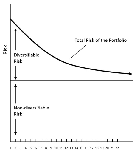
The amount of risk reduction achieved by diversiﬁcation also depends on the number of stocks in the portfolio. As the number of stocks increases, the diversifying effect of each additional stock diminishes as shown in the ﬁgure below:

Risk Reduction through Diversification

As the ﬁgure indicates, the major beneﬁts of diversiﬁcation are obtained with the ﬁrst 10 to 12 stocks, provided they are drawn from industries that are not closely related. Additions to the portfolio beyond this point continue to reduce total risk but the beneﬁts are diminishing.

From the ﬁgure it is also apparent that it is the diversiﬁable risk that is being reduced unlike the non-diversiﬁable risk which remains constant whatever your portfolio is. What are diversiﬁable and non-diversiﬁable risks? The risk of any individual stock can be separated into two components: non-diversiﬁable and diversiﬁable risk.

Non-diversiﬁable risk is that part of total risk (from various sources like interest rate risk, inﬂation risk, ﬁnancial risk, etc.) that is related to the general economy or the stock market as a whole and hence cannot be eliminated by diversiﬁcation. Non-diversiﬁable risk is also referred to as market risk or systematic risk.

Diversiﬁable risk on the other hand, is that part of total risk that is speciﬁc to the company or industry and hence can be eliminated by diversiﬁcation. Diversiﬁable risk is also called unsystematic risk or speciﬁc risk.

Let us take a look at some of the factors that give rise to diversiﬁable and non-diversiﬁable risk.

Non-diversifiable or Market Risk Factors

Major changes in tax rates
War & other calamities
An increase or decrease in inﬂation rates
A change in economic policy
Industrial recession
An increase in international oil prices, etc.

Diversifiable or Specific Risk Factors

Company strike
Bankruptcy of a major supplier
Death of a key company officer
Unexpected entry of new competitor into the market etc.

Risk of Stocks in a Portfolio
How do you measure the risk of stocks in a portfolio? You can think of a portfolio‘s standard deviation as a good indicator of its risk to the extent that if addition of a stock to the portfolio increases the portfolio’s standard deviation, the stock adds risk to the portfolio. But the risk that a stock adds to a portfolio will depend not only on the stock’s total risk, its standard deviation, but on how that risk breaks down into diversiﬁable and non-diversiﬁable risk. If an investor holds only one stock, there is no question of diversiﬁcation, and his risk is therefore, the standard deviation of the stock. For a diversiﬁed investor, the risk of a stock is only that portion of the total risk that cannot be diversiﬁed away or its non-diversiﬁable risk. How do you measure non-diversiﬁable or market risk? It is generally measured by Beta (β) coefficient. Beta measures the relative risk associated with any individual portfolio as measured in relation to the risk of the market portfolio. The market portfolio represents the most diversiﬁed portfolio of risky assets an investor could buy since it includes all risky assets. This relative risk can be expressed as:

Formula of Relative Risk

Thus, the beta coefficient is a measure of the non-diversiﬁable or systematic risk of an asset relative to that of the market portfolio. A beta of 1.0 indicates an asset of average risk. A beta coefﬁcient greater than 1.0 indicates above-average risk — stocks whose returns tend to be more risky than the market. Stocks with beta coefficients less than 1.0 are of below average risk i.e., less riskier than the market portfolio. An important point to note here is that in the case of the market portfolio, all the possible diversiﬁcation has been done — thus the risk of the market portfolio is non-diversiﬁable which an investor cannot avoid. Similarly, as long as the asset’s returns are not perfectly positively correlated with returns from other assets, there will be some way to diversify away its unsystematic risk. As a result beta depends only on non-diversiﬁable risks.

The beta of a portfolio is nothing but the weighted average of the betas of the securities that constitute the portfolio, the weights being the proportions of investments in the respective securities. For example, if the beta of a security A is 1.5 and that of security B is 0.9 and 60% and 40% of our portfolio is invested in the 2 securities respectively, the beta of our portfolio will be 1.26 (1.5 x 0.6 + 0.9 x 0.4).

Measurement of Beta
The systematic relationship between the return on the security or a portfolio and the return on the market can be described using a simple linear regression, identifying the return on a security or portfolio as the dependent variable kj and the return on market portfolio as the independent variable km, in the single-index model or market model developed by William Sharpe. This can be expressed as:

kj = αj + βjkm + ej

The beta parameter βj in the model represents the slope of the above regression relationship and as explained earlier, measures the responsiveness of the security or portfolio to the general market and indicates how extensively the return of the portfolio or security will vary with changes in the market return. The beta coefficient of a security is defined as the ratio of the security’s covariance of return with the market to the variance of the market.

The Capital Asset Pricing Model (CAPM)
The CAPM developed by William F Sharpe, John Lintner and Jan Mossin is one of the major developments in financial theory. The CAPM establishes a linear relationship between the required rate of return of a security and its systematic or undiversifiable risk or beta.

The CAPM is represented mathematically by

kj = Rf + Bj (km - Rf)

where,
kj = expected or required rate of return on security j
Rf = risk-free rate of return
Bj = beta coefﬁcient of security j
km = return on market portfolio.

Assumptions:

Investors are risk-averse and use the expected rate of return and standard deviation of return as appropriate measures of risk and return for their portfolio. In other words, the greater the perceived risk of a portfolio, the higher return a risk-averse investor expects to compensate the risk.
Investors make their investment decisions based on a single-period horizon i.e., the next immediate time period.
Transaction costs in ﬁnancial markets are low enough to ignore and assets can be bought and sold in any unit desired. The investor is limited only by his wealth and the price of the asset.
Taxes do not affect the choice of buying assets.
All individuals assume that they can buy assets at the going market price and they all agree on the nature of the return and risk associated with each investment.

The assumptions listed above are somewhat limiting but the CAPM enables us to be much more precise about how trade-offs between risk and return are determined in ﬁnancial markets.

In the CAPM, the expected rate of return can also be thought of as a required rate of return because the market is assumed to be in equilibrium. The expected return is the return from an asset that investors anticipate or expect to earn over some future period. The required rate of return for a security is deﬁned as the minimum expected rate of return needed to induce an investor to purchase it.

What do investors require (expect) when they invest? First of all, investors can earn a riskless rate of return by investing in riskless assets like treasury bills. This risk-free rate of return is designated Rf and the minimum return expected by the investors. In addition to this, because investors are risk-averse, they will expect a risk premium to compensate them for the additional risk assumed in investing in a risky asset.

Required Rate of Return = Risk-free rate + Risk premium.

The CAPM provides an explicit measure of the risk premium. It is the product of the Beta for a particular security j and the market risk premium km - Rf

Risk premium = βj (km - Rf)

This beta coefﬁcient ‘βj’ is the non-diversiﬁable risk of the asset relative to the risk of the market. If the risk of the asset is greater than the market risk. i.e. β exceeds 1.0, the investor assigns a higher risk premium to asset than to the market.

The Security Market Line (SML)
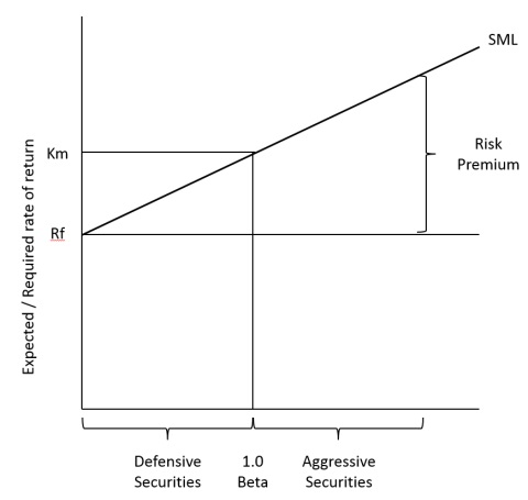
You can plot the relationship between the required rate of return (kj) and non-diversiﬁable risk (beta) as expressed in CAPM to produce a graph of the SML as shown below:

Risk and Return

As per the CAPM assumptions, any individual security’s expected return and beta statistics should lie on the SML. The SML intersects the vertical axis at the risk-free rate of return Rf and km - Rf is the slope of the SML.

Since all securities are expected to plot along the SML, the line provides a direct and convenient way of determining the expected/required return of a security if you know the beta of the security. The SML can also be used to classify securities. Those with betas greater than 1.00 and plotting on the upper part of the SML are classiﬁed as aggressive securities while those with betas less than 1.00 and plotting on the lower part of the SML can be classiﬁed as defensive securities which earn below-average returns.

One of the major assumptions of the CAPM is that the market is in equilibrium and that the expected rate of return is equal to the required rate of return for a given level of market risk or beta. In other words, the SML provides a framework for evaluating whether high-risk stocks are offering returns more or less in proportion to their risk and vice-versa. Let us see how we can appraise the value securities using CAPM, and the SML.

Summary:

An investment portfolio refers to the group of assets that is owned by an investor.
Returns on stocks do not move in perfect tandem means that risk can be reduced by diversiﬁcation.
The amount of risk reduction depends on the degree of positive correlation between stocks.
As the number of stocks increases, the diversifying effect of each additional stock diminishes.
The portfolio‘s standard deviation as a good indicator of its risk.
Beta measures the relative risk associated with any individual portfolio as measured in relation to the risk of the market portfolio.
The Capital Asset Pricing Model (CAPM) establishes a linear relationship between the required rate of return of a security and its systematic or undiversifiable risk or beta.

Financial Risk Management

In this chapter, you will:

Understand the various types of financial risks.

Since time immemorial, human beings have tried to manage risks they faced in their day-to-day life. Keeping inﬂammable material away from ﬁre, saving for possible future needs, creation of a legal will are all examples of an attempt at managing risk. Risk is the possibility of the actual outcome being different and adverse from the expected outcome. It includes both the downside and the upside potential. Downside potential is the possibility of the actual results being adverse compared to the expected results. On the other hand, upside potential is the possibility of the actual results being better than the expected results.

Although the terms risk and uncertainty are often used interchangeably, they are in fact not synonymous. There is a clear distinction between certainty, uncertainty and risk. Certainty is the situation where it is known what will happen and the happening or non-happening of an event carries a 100% probability. Risk is the situation when there are a number of speciﬁc, probable outcomes, but it is not certain as to which one of them will actually happen. Uncertainty is where even the probable outcomes are unknown. It reﬂects a total lack of knowledge of what may happen. Risk is generally measured using the concept of standard deviation.

A corporate’s aim is to create wealth for its shareholders. This wealth is reﬂected in the market value of its shares. Hence, for a company the risk faced is reﬂected in the possibility of the actual market value of its shares being different from the expected market value. As the market value of a ﬁrm’s shares is closely related to the proﬁt it earns, corporate risk can also be termed as the possibility of a company’s actual Proﬁts After Tax (PAT) being different from the expected PAT. For a corporate, downside risk may stem from the possibility of either costs being higher than expected, or revenues being lower than expected. Similarly the upside risk may result from either the possibility of costs being lower than expected, or the possibility of revenues being higher than expected.

Sources of Risks
The proﬁts of a company are at risk from different sources. The various risks faced by a ﬁrm are interest rate risk, exchange risk, default risk, liquidity risk, business risk, ﬁnancial risk, market risk and marketability risk. While the list is not exhaustive, it does cover the most signiﬁcant risks.

Interest Rate Risk:
Interest rate risk is the risk of an adverse effect of interest rate movements on a ﬁrm’s proﬁts or balance sheet. Interest rates affect a ﬁrm in two ways — affecting the proﬁts and affecting the value of its assets or liabilities. For example, a ﬁrm that has borrowed money on a ﬂoating rate basis faces the risk of lower proﬁts in an increasing interest rate scenario.

Exchange Risk:
Exchange risk is the risk of the possibility of adverse effect on the value of a ﬁrm’s assets, liabilities or income, as a result of exchange rate movements. Adverse movements in exchange rate can affect a ﬁrm’s proﬁts, assets or liabilities, even if it is not operating in foreign markets. This happens due to the inter-linkages between the various markets.

Default Risk:
Default risk is the risk of non-recovery of sums due from outsiders, which may arise either due to their inability to pay or unwillingness to do so. This risk has to be considered when credit is extended to any party.

Liquidity Risk:
Liquidity risk refers to the risk of a possible bankruptcy arising of the ﬁrm to meet its ﬁnancial obligations. There is a misconception that a proﬁtable ﬁrm will have little or no liquidity risk. It is possible that a ﬁrm may be very proﬁtable but may have a severe liquidity crunch because it has blocked its money in illiquid assets.

Business Risk:
Business risk is the risk faced by a business from its external and internal environment. The risk may come from internal factors like labour strike, death of key personnel, machinery breakdown, or external factors like government policy, changes in customer preferences, etc.

Financial Risk:
Financial risk refers to the risk of bankruptcy arising from the possibility of a ﬁrm not being able to repay its debts on time. Higher the debt-equity ratio of a ﬁrm, higher the ﬁnancial risk it faces. Liquidity risk and wrong capital structure are the prime reasons for ﬁnancial risk.

Market Risk:
Market risk is the risk that arises when the value of a ﬁrm’s investments go down as a result of market movements. It is also referred to as price risk. Market risk cannot be distinctly separated from other risks deﬁned above, as it results from interplay of these risks. Interest rate risk and exchange risk contribute most to the presence of market risk.

Marketability Risk:
This is the risk of the assets of a ﬁrm not being readily marketable. The situation of having non-marketable asset-s may or may not be linked to a need for funds. When such assets are required to be sold due to a need for funds, their non-marketability may lead to liquidity risk.

Summary:

Risk is the situation when there are a number of speciﬁc, probable outcomes, but it is not certain as to which one of them will actually happen.
Interest rate risk is the risk of an adverse effect of interest rate movements on a ﬁrm’s proﬁts or balance sheet.
Exchange risk is the risk of the possibility of adverse effect on the value of a ﬁrm’s assets, liabilities or income, as a result of exchange rate movements.
Default risk is the risk of non-recovery of sums due from outsiders, which may arise either due to their inability to pay or unwillingness to do so.
Liquidity risk refers to the risk of a possible bankruptcy arising of the ﬁrm to meet its ﬁnancial obligations.
Business risk is the risk faced by a business from its external and internal environment.
Financial risk refers to the risk of bankruptcy arising from the possibility of a ﬁrm not being able to repay its debts on time.
Market risk is the risk that arises when the value of a ﬁrm’s investments go down as a result of market movements.
Marketability is the risk of the assets of a ﬁrm not being readily marketable.

Risk Management Process

In this chapter, you will:

Understand the various approaches to Risk Management
Understand the risk management process
Understand the process of evaluating risk

Corporate risk management refers to the process of a company attempting to managing its risks at an acceptable level. It is a scientiﬁc approach to deal with various kinds of risks a corporate faces. According to Mark Dorfman, risk management is “the logical development and execution of a plan to deal with potential losses”. It is a dynamic process which changes according to the evolving scenario. The aim of risk management is to maintain overall and speciﬁc risks at the desired levels, at the minimum possible cost.

There is a misconception that the goal of risk management is the complete elimination of risk. In reality, risk management aims at ensuring that risk remains at the desired and acceptable level, or within an acceptable range. Complete elimination of risk can take place only when no business activity is undertaken. In fact, the returns earned on government securities, which is generally referred to as the risk-free rate of return, is also not free from risks. The only risk such investments do not carry is default risk. In order to earn returns, it is essential to bear some risks. Risk management only aims at bringing the risk to a level that is in line with the returns expected to be generated by the investment. As the factors affecting risk change continuously, the risk faced by a ﬁrm also changes. Therefore, a company needs to continuously evaluate its risk level and make an attempt to bring it to the targeted level. This may even include efforts at increasing risk when it is below the targeted level.

Approaches to Risk Management
Following are the different approaches to managing risks:

Risk Management Techniques

Risk Avoidance
An extreme way of managing risk is to avoid it altogether. This can be done by not undertaking the activity that entails risk. For example, a corporate may decide not to invest a particular industry because the risk involved exceeds its risk bearing capacity. Though this approach is relevant under certain circumstances, it is more of an exception rather than a rule. It is neither prudent, nor possible to use it for managing all kinds of risks. The use of risk avoidance for managing all risks would result in no activity taking place, as all activities involve risk, while the level may vary.

Loss Control
Loss control refers to the attempt to reduce either the possibility of a loss or the quantum of loss. This is done by making adjustments in the day-to-day business activities. For example, a ﬁrm having ﬂoating rate liabilities may decide to invest in ﬂoating rate assets to limit its exposure to interest rate risk.

Combination
Combination refers to the technique of combining more number of business activities in order to reduce the overall risk of the ﬁrm. It is also referred to as aggregation or diversiﬁcation. It entails entering into more than one business, and these different businesses have the least possible correlation with each other. The absence of a possible correlation results in at least some of the businesses generating proﬁts at any given time. Thus, it reduces the possibility of the ﬁrm facing losses.

Separation
Separation is the technique of reducing risk through separating parts of businesses or assets or liabilities. For example, a ﬁrm having two highly risky businesses with a positive correlation may spin-off one of them as a separate entity in order to reduce its exposure to risk. Or, a company may locate its inventory at a number of places instead of storing all at one place, in order to reduce the risk of destruction by ﬁre.

Risk Transfer
Risk is transferred when the ﬁrm, originally exposed to a risk, transfers it to another party which is willing to bear the risk. This may be done in three ways. The ﬁrst is to transfer the asset itself. For example, a ﬁrm into a number of businesses may sell—off one of them to another party, and thereby transfer the risk involved in it. The second way is to transfer the risk without transferring the title of the asset or liability. This may be done by hedging through various derivative instruments like forwards, futures, swaps and options. The third way is through arranging for a third party to pay for losses if they occur, without transferring the risk itself. This is referred to as risk ﬁnancing. This may be achieved by buying insurance.

Risk Retention
Risk is retained when nothing is done to avoid, reduce, or transfer it. Risk may be retained consciously because the other techniques of managing risk are either too costly or because it is not possible to employ other techniques. Risk may even be retained unconsciously when the presence of risk is not recognized. It is very important to distinguish between the risks that a ﬁrm is ready to retain and the ones it wants to offload using risk management techniques.

Risk Sharing
This technique is a combination of risk retention and risk transfer. Under this technique, a particular risk is managed by retaining a part of it and transferring the rest to a party willing to bear it. For example, a ﬁrm and its supplier may enter into an agreement, whereby if the market price of the commodity exceeds a certain price in the future, the seller foregoes a part of the beneﬁt in favour of the ﬁrm, and if the future market price is lower than a predetermined price, the ﬁrm passes on a part of the beneﬁt to the seller.

Risk Management Process
Risk management needs to be looked at as an organizational approach, as management of risks independently cannot have the desired effect over the long-term. This is especially necessary as risks result from various activities in the firm, and the personnel responsible for the activities do not always understand the risk attached to them. Risk management function involves a logical sequence of steps. These steps are:

Determining Objectives:
Determination of objectives is the ﬁrst step in the risk management function. The objective may be to protect proﬁts, or to develop competitive advantage. The management needs to decide the objective of risk management, so that the risk manager may fulfil his responsibilities in accordance with the set objectives.

Identifying Risks:
Every organization faces different risks, based on its business, the economic, social and political factors, the features of the industry it operates in like the degree of competition, the strengths and weaknesses of its competitors, availability of raw material, factors internal to the company like the competence and outlook of the management, state of industry relations, dependence on foreign markets for inputs, sales, or ﬁnances, capabilities of its staff, besides other innumerable factors. Each corporate needs to identify the possible sources of risks and the kinds of risks it faces. For this, the risk manager needs to develop a fundamental understanding of all the ﬁrm’s activities and the external factors that contribute to risk.

Risk Evaluations:
Once the risks are identiﬁed, they need to be evaluated for ascertaining their signiﬁcance. The signiﬁcance of a particular risk depends upon the size of the loss that it may result in, and the probability of the occurrence of such loss. On the basis of these factors, the various risks faced by the corporate need to be classiﬁed as critical risks, important risks and not-so—important risks. Critical risks are those that may result in bankruptcy of the ﬁrm. Important risks are those that may not result in bankruptcy, but may cause severe ﬁnancial distress. The not-so-important risks are those that may result in losses which the ﬁrm may easily bear in the normal course of business.

Development of Policy:
Based on the risk tolerance level of the ﬁrm, the risk management policy needs to be developed. The time-frame of the policy should be comparatively long, so that the policy is relatively stable. A policy generally takes the form of a declaration as to how much risk should be covered; or in other words, how much risk the ﬁrm is ready to bear. For example, a policy may specify that a speciﬁc percentage, say 50%, of all risks are to be covered or that not more than a speciﬁc sum can be at risk at any given point of time.

Development of Strategy:
Based on the policy, the ﬁrm then needs to develop the strategy to be followed for managing risk. The tenure of a strategy is shorter than a policy, as it needs to factor-in various variables that keep changing. A strategy is essentially an action plan, which speciﬁes the nature of risk to be managed and the timing. It also speciﬁes the tools, techniques and instruments that can be used to manage these risks. A strategy also deals with tax and legal problems. It may specify whether it would be more beneﬁcial for a subsidiary to manage its own risk, or to shift it to the parent company. It may also specify as to how it will be most beneﬁcial to shift the losses to a branch located at a particular location. Another important issue that needs to be speciﬁed by the strategy is, whether the company would try to make proﬁts out of risk management (from active trading on the derivatives market) or would it stick to covering the existing risks.

Implementation:
Once the policy and strategy are in place, they are to be implemented for actually managing the risks. This is the operational part of risk management. It includes ﬁnding the best deal in case of risk transfer, providing for contingencies in case of risk retention, designing and implementing risk control programs, etc. It also includes taking care of the details in the operational part, like the back ofﬁce work, ensuring that the controls are complied with, etc.

Review:
The function of risk management needs to be reviewed periodically, depending on the costs involved. The factors that affect the risk management decisions keep changing, thus necessitating the need to monitor the effectiveness of the decisions taken previously. Sometimes, the decisions taken earlier may not prove to be correct, or the changing circumstances may make some other option, more effective. A periodic review ensures that the risk management function remains ﬂexible, and the tools, techniques and instruments used for managing risk change according to the changing circumstances. In effect, review helps the risk manager analyze whether the risk management function is achieving the set objectives or not and to ﬁnd an alternative course of action if the results are not in accordance with expectations.

Summary:

Risk avoidance can be done by not undertaking the activity that entails risk.
Loss control refers to the attempt to reduce either the possibility of a loss or the quantum of loss.
Combination refers to the technique of combining more number of business activities in order to reduce the overall risk of the ﬁrm.
Separation is the technique of reducing risk through separating parts of businesses or assets or liabilities.
Risk is transferred when the ﬁrm, originally exposed to a risk, transfers it to another party which is willing to bear the risk.
Risk is retained when nothing is done to avoid, reduce, or transfer it.
Risk sharing technique is a combination of risk retention and risk transfer.
Risk management involves:
- Determining objectives and
- Identifying risks
Risk evaluation involves:
- Development of policy
- Deployment of strategy
- Implementation and
- Review

Your Free Premium MBA Training
Table of Contents

Training Material for Your
MBA Finance™ Degree

MBA Finance™ Training

Nature and Importance of the Finance Function

Functions of the Finance Manager

Interface Between Finance and Other Business Functions

Environment of Corporate Finance

Time Value for Money

The Measure of Return

Sources of Financial Risks

Financial Portfolios and Risks

Financial Risk Management

Risk Management Process

Your Free Premium MBA Training
Table of Contents

MBA Leadership™ Training

MBA Management™ Training

MBA Sales™ Training

MBA Human Resources™ Training

MBA Finance™ Training

MBA Marketing™ Training

MBA Business Strategy™ Training

MBA Recruitment™ Training

Training Material for YourMBA Finance™ Degree

MBA Finance™ Training

Nature and Importance of the Finance Function

Functions of the Finance Manager

Interface Between Finance and Other Business Functions

Environment of Corporate Finance

Time Value for Money

The Measure of Return

Sources of Financial Risks

Financial Portfolios and Risks

Financial Risk Management

Risk Management Process

Your Free Premium MBA TrainingTable of Contents

MBA Leadership™ Training

MBA Management™ Training

MBA Sales™ Training

MBA Human Resources™ Training

MBA Finance™ Training

MBA Marketing™ Training

MBA Business Strategy™ Training

MBA Recruitment™ Training

Training Material for Your
MBA Finance™ Degree

Your Free Premium MBA Training
Table of Contents